:: Stochastic differential equations ::

Download [ex03sde.sce] - Scilab file for this exercise session

• Nonrandom function can be given as a solution to an ordinary differential equation - we are given a relation between the differential of the function as the differential of time. For example: dx(t)=x(t) dt, together with initial condition x(0) defines a (deterministic, i.e., non-random) function x(t).
  
  
• Analogy for stochastic functions - relation between the differential of the function, of time and of a Wiener process (dw). In this way we obtain so called stochastic differential equations. Their solution is a stochastic process. For example:
  • dx=2dt+3dw, initial condition x(0)=0 - this is a Brownian motion x(t)=2t+3w(t)
  • dx=2dt+3dw, initial condition x(0)=1 - a shifted Brownian motion, starts from 1: x(t)=1+2t+3w(t)
  • dx=10[1-x(t)] dt + 0.25 dw(t), x(0)=0.5 - can be written expilicitly too, but this expression is more compicated. However, we can get a good idea about a process from its simulations.
  
  
• So, let us consider the process
  
  where are positive constants. It is called an Ornstein-Uhlenbeck process.
  
  The simplest method, how to obtain an approximation of a solution to a stochastic differential equation, is to replace the differentials by differences (analogy of Euler method for ordinary differential equations) - this approach is called Euler-Maruyama method:
  
  
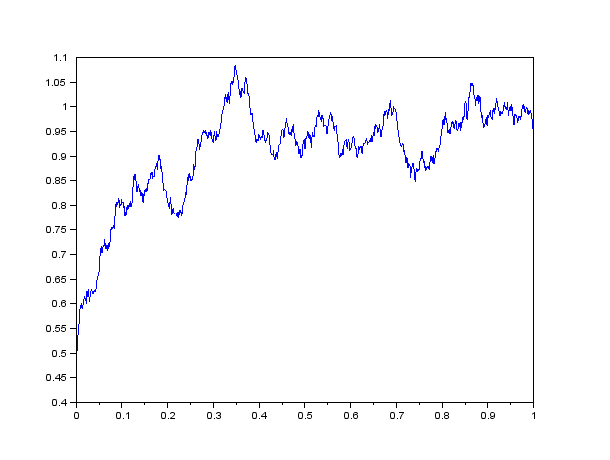
  Sample result: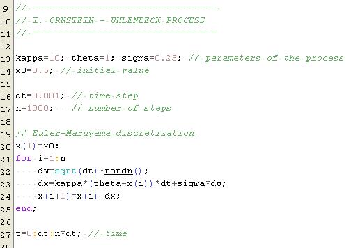
  
  
  
• Terminology: Deterministic part of the process (coefficient at dt) - drift, stochastic part (coefficient at the Wiener process differential dw) - volatility.

:: Exercises (1) ::

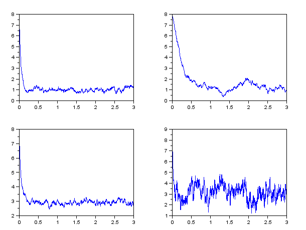
1. Write a Scilab function, which generates a vector with a sample path of an Ornstein-Uhlenbeck process for the given initil value, parameters of the process and time ticks. Plot some trajectories of an Ornstein-Uhlenbeck process with selected parameters and note the changes depending on parameter values.
   
   Add the following parameter sets to their trajectories:
   • = 20, = 1, = 1
   • = 3, = 1, = 1
   • = 20, = 3, = 5
   • = 20, = 3, = 1
   
   
   
2. Ornstein-Uhlenbeck process is used for example in interest rates modelling. Vasicek model assumes that the instantaneous interest rate (practically - when analysing real data - interest rate with a short maturity) follows an Ornstein-Uhlenbeck process.
   
   In paper Athanasios Episcopos: Further evidence on alternative continuous time models of the short-term interest rate. Journal of International Financial Markets, Institutions and Money 10 (2000) 199-212 the author estimates interest rate models. The general model which he considered is
   
   Special choices of some of the parameters lead to concrete models, one of them is also the Vasicek model. Results for New Zealand (estimated are based on monthly data, from April 1986 - April 1998) can be seen in the following table, taken from the paper: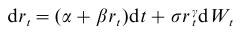
   
   Source: (Episcopos, 2000)
   
   
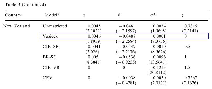
   • The process is written in another parametization. Write it in terms of the parameters , , . What is the equilibrium level, to which the interest rate reverts?
   • Simulate future behaviour of the interest rate using the estimated parameters of the Vasicek model. Into one graph, plot several sample paths starting from the same initial value.

---

---