Pricing American options
:: Numerical solution ::
- We need to ensure that the derivative price does not fall under the payoff - that would be an arbitrage.
- We know:
- The price of a European call option on a stock which does not pay dividends lies above the payoff.
- The price of a European call option on a stock which pays dividends always crosses the payoff.
- The price of a European put (regardless of whether the stock pays dividends or not) always crosses thepayoff.
- Therefore: For an American call on a stock that does not pay dividends and an American put on an arbitraty stock, the price is different from their European counterpart.
- The derivative price smoothly pastes to the payoff - theorem from the lectures
- From the lectures - algorithm for a call option:
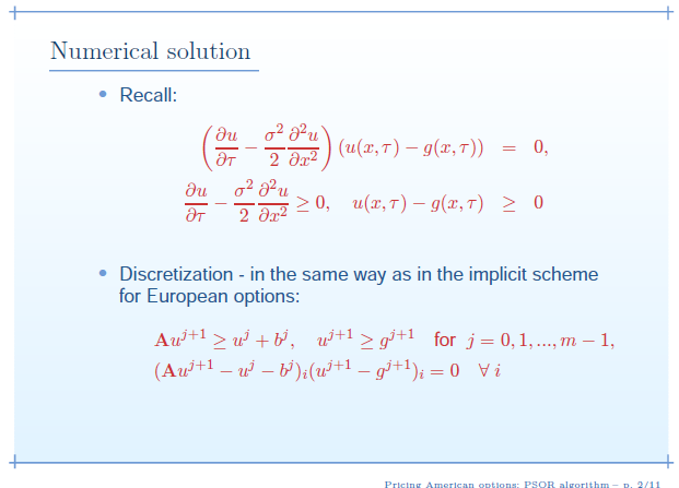
- Formulation in terms of a free boundary problem.
- Transformation to a linear complementarity problem (on a fixed domain - for all positive stock prices)
- The same sequence of transformations as in the case of a Europea option (there we obtained a heat equation)
- We continue:
- Discretization:
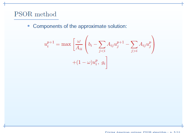
- Numerical scheme for solving the discrete problem:
- Discretization:
:: Comparison of numerical pricing: European vs. American option ::
European option - algorithm for the transformed function u- We compute the boundary conditions and insert them into the solution matrix.
- We compute the initial condition and insert it into the solution matrix.
- Computation of the next time level - SOR method:
- Initial approximation: we can take the values from the previous time level
- Condition for stopping the iterations - norm of the residue
- Computation of a new iteration using the SOR method - we repeat until the condition for stopping the iteration is not satisfied, the we move to the next time level
- We compute the boundary conditions. The solution has to lie above the transformed payoff => we compute max(boundary condition, transformed payoff) and insert it into the solution matrix.
- We compute the initial condition and insert it into the solution matrix.
- Computation of the next time level - - PSOR method (projected SOR method)
- Initial approximation - we want one that is close to solution, so that we do not have to compute many iterations: we compare the values from the previous time level with the transformed payoff => we take max(previous time level, transformed payoff)
- Condition for stopping the iterations - norm of a residue cannot be used, since we do not compute a solution to a system of equations, we use the difference of two subsequent iterations
- Computation of a new iteration using the PSOR method - we compute the i-th elemts of the vector using SOR method and compare it with the transformed payoff => we take max(SOR iteration, transformed payoff) and compute the next element - we repeat until the condition for stopping the iteration is not satisfied, the we move to the next time level
:: Exercise ::
Implement the algorithm above.
:: Practice problems ::
- How does the algorithm change for put option?
-
The stock price S follows a geometrical Brownian motion with parameters
 =0.20,
  =0.40. The stock does not pay dividends. Interest rate equals 10 percent. Compute the price of a put option with expiration in half a year and exercise pirce 10 USD for the following stock pricces: 0, 2, 4, 6, 8, 10, 12, 14, 16
USD. Give the results to 4 decimal places.
=0.40. The stock does not pay dividends. Interest rate equals 10 percent. Compute the price of a put option with expiration in half a year and exercise pirce 10 USD for the following stock pricces: 0, 2, 4, 6, 8, 10, 12, 14, 16
USD. Give the results to 4 decimal places.
Belowe are the results for an option with expiration in 3 months (the remaining parameters are the same); they can be useful when testing the parameters of the numerical schemes and method for computing the option prices for those stock values which are not grid points.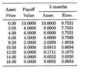
Financial derivatives - exercises, 2014
Beáta Stehlíková, FMFI UK Bratislava
E-mail: stehlikova@pc2.iam.fmph.uniba.sk
Web: http://pc2.iam.fmph.uniba.sk/institute/stehlikova/
Beáta Stehlíková, FMFI UK Bratislava
E-mail: stehlikova@pc2.iam.fmph.uniba.sk
Web: http://pc2.iam.fmph.uniba.sk/institute/stehlikova/