:: Stochastic character of financial variables ::

• From the trajectories of stock prices (also other financial variables - interest rate, exchange rates, etc.) we see that it cannot be described by a deterministic function. Therefore, stochastic processes are used in the modelling. .
  
  
• Left: trend (stock price, 5 years time frame), right: fluctuations (stock price, time frame of a couple of hours)
  
  
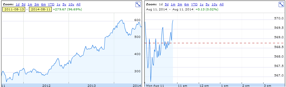  Source: http://finance.google.com

:: Wiener process ::

• The basic process, used to derive more complicated ones, is a Wienerov proces. Recall its definition:
  
  Random process {W(t), t0} is called a Wiener process, if

  • the increments W(t+) -  W(t) have a normal distribution with zero expected value and variance equal to ,
  • for every partition 0 = t₀  t₁  ...   t_n, the increments W_ti+1 - W_ti nare independent random variables, with distribution given in the previous points ,
  • W(0)=0,
  • trajectories are continuous.
  In what follows, we denote a Wiener process by w.
  
  
• How to obtain a sample path (trajectory) of a Wiener process
  • We will generate an approximation - values at discrete points of the form (time, value of the process) which we join by line segments.
  • The times will be 0,,2, . . ., where is a sufficiently small time step.
  • Value at time 0 is equal to 0.
  • Increment on the interval [k, (k + 1)] is a random variable with zero expected value and variance equal to .
  
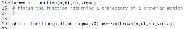
  In R: download the file ex02_wiener.R which contains also the following function:
  
  
  
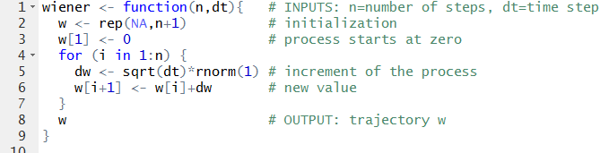
  Note that it is not computationally optimal - generally, loops are not the best idea - but it is illustrative (and of course you can modify it to make it more efficient).
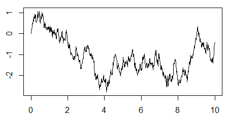
  Now we can plot a trajectory:
  
  

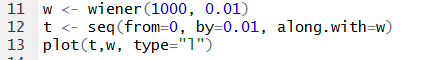
  We get something like:

  
  
  

:: Exercises (1) ::

1. Add more trajectories of a Wiener process into one plot. When doing this, we may encounter something like this:
   
   The new trajectory does not fit into the bounds determined when displaying the first one. Compute the bounds for the vertical axis, such that you have a 95 percent probability that the end of the trajectory will be withing these bounds.
   
   Naturally, this doesn't necessarily mean that the whole trajectory will fit. You will explore the maximum of a Wiener process in practice problems.
   
   
2. Simulate the values of the random variable w(1)+w(2) and make a histogram of its values. Compute the probability distribution of this random variable and check your answer with the histogram from the simulations.

:: Brownian motion and geometric Brownian motion ::

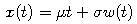
• By adding a linear trend to a multiple of a Wiener process:
  
  we obtain a process which is known as a Brownian motion.

• If the parameter is zero, the resulting graph is a line. For a nonzero value of , there are random fluctuations added to this linear trend.

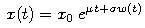
• Geometric Brownian motion is defined as:
  
  where x₀ is the value of the process at time 0.

• In R: Finish the definition of a Brownian motion. It will also allow you to use the function for a geometric Brownian motion.
  

:: Exercises (2) ::

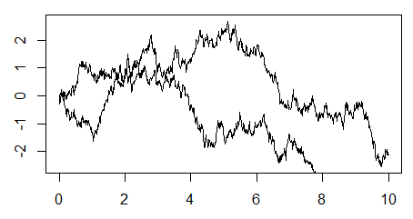
1. Plot some trajectories of a Brownian motion into one figure and add the expected value. A sample output:
   
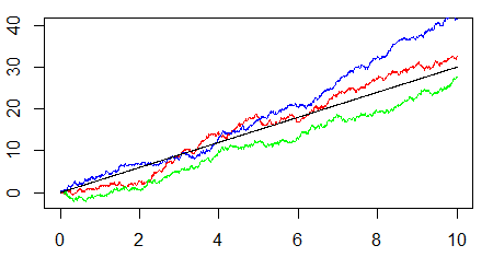
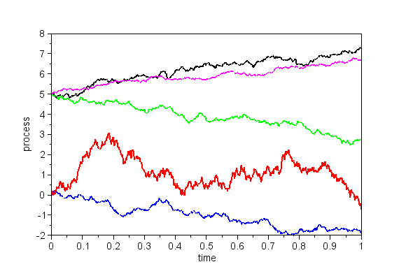
2. Modify parameters of a Brownian motion and note the influence on typical trajectories. Then, add the processes
   • x₁(t)=w(t)
   • x₂(t)=3*w(t)
   • x₃(t)=5+2*t+w(t)
   • x₄(t)=5+2*t+0.5*w(t)
   • x₅(t)=5-3*t+w(t)
   to their sample paths below:
   
   
   
3. Plot some trajectories of a geometric Brownian motion into one figure and add the expected value.

:: Exercises (3) ::

1. Suppose that the stock price follows a GBM with parameters  = 0.30,  = 0.25 and that its current price is 150 USD.
   • Plot the probability density function of the stock price in one month.
   • Compute the probability that the price in one month will be lower than 140 USD.
   • What it expected value of the 1/4-year return? What is the probability that this return will be negative?

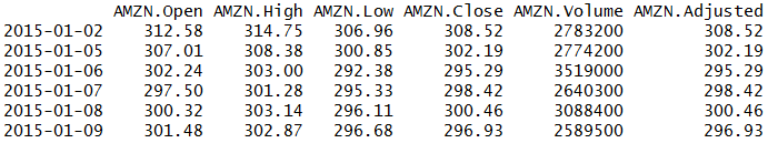
:: Estimating the parameters of the GBM from stock prices in R ::

• We will use the quantmod package which allows us to conveniently download the data directly to R:
  
  The header of our data:
  
• The estimation will be based on returns computed from the end of the day adjusted prices:
  
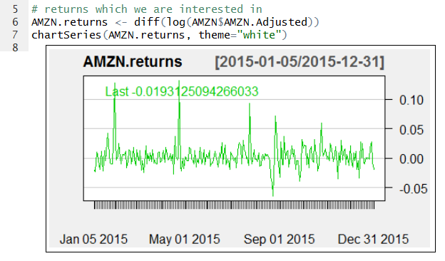
• Download the file ex02_stocks.R and finish the script by computing the esimate of the stock volatility.

:: Practice problems ::

1. Let w be a Wiener process; define B(t) = w(t) - t w(1) for time t in interval [0, 1]. It is known as Brownian bridge.
   • Plot some sample paths of the process and explain its name.
   • Compute its variance at time t and sketch its behaviour as a function of time. To check your computation - what does the result have to be for t=0 and t=1?
   
   
2. Denote by t_M the time, in which the sample path of the Wiener process achieved its maximum on the time interval [0, 1]. Plot a histogram by simulating the realizations of the random variable t_M.
   
   A trajectory of a Wiener process and corresponding value of t_M is shown below, together with a sample histogram.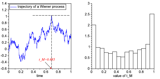
   
   
   
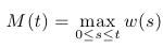
3. Define the process so that its value at time t is the maximum of a Wiener process on the interval [0,t]:
   
   A sample trajectory is depicted on the following plot:
   
   Using simulations estimate the distribution of this so-called running maximum at time t=1 and its expected value. (Here it is wirth noting that computation of the maximum using values from a discrete time set is an underestimate of the real maximum of the trajectory. Therefore, in order to obtain a more precise estimate of the expected value it is not sufficient only to simulate a large number of trajectories, but also to use a sufficiently small time step.)
   
   
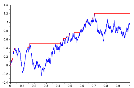
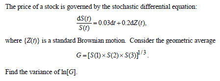
4. From Society of Actuaries exam:
   
   We have seen some problems from the exam on the lecture, also here it is actually a multiple-choice question and the choices are: 0.03, 0.04, 0.05, 0.06, 0.07.
   
   
5. Define a process:
   
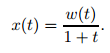
   • Plot some trajectories of the process. (Plot more trajectories, so that the typical behaviour of the process can be better observed.) How does the variance change in time? A sample graph:
     
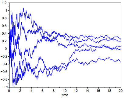
   • Compute the mean and variance of the process analytically. At which time achieves the variance its maximum? What is its limit as time approaches infinity? Compare these results with the simulations of the trajectories.
   • Add 95 percent confidence interval for the value at the given time to the graph.

---

---