Random processes II.
Stochastic differential equations
:: Stochastic differential equations ::
Download ou.R - R file for this exercise
- Nonrandom function can be given as a solution to an ordinary differential equation - we are given a relation between the differential of the function as the differential of time. For example: dx(t)=x(t) dt, together with initial condition x(0) defines a (deterministic, i.e., non-random) function x(t).
- Analogy for stochastic functions - relation between the differential of the function, of time and of a Wiener process (dw). In this way we obtain so called stochastic differential equations. Their solution is a stochastic process. For example:
- dx=2dt+3dw, initial condition x(0)=0 - this is a Brownian motion x(t)=2t+3w(t)
- dx=2dt+3dw, initial condition x(0)=1 - a shifted Brownian motion, starts from 1: x(t)=1+2t+3w(t)
- dx=10[1-x(t)] dt + 0.25 dw(t), x(0)=0.5 - can be written expilicitly too, but this expression is more compicated. However, we can get a good idea about a process from its simulations.
- So, let us consider the process
where
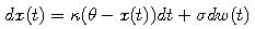
 are positive constants. It is called an Ornstein-Uhlenbeck process.
The simplest method, how to obtain an approximation of a solution to a stochastic differential equation, is to replace the differentials by differences (analogy of Euler method for ordinary differential equations) - this approach is called Euler-Maruyama method:
Sample result: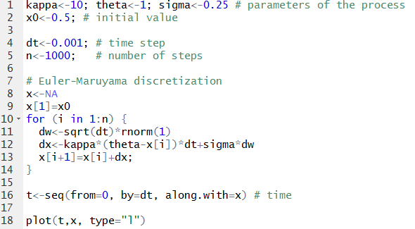
- Terminology: Deterministic part of the process (coefficient at dt) - drift, stochastic part (coefficient at the Wiener process differential dw) - volatility.
:: Exercises (1) ::
- Write a function, which generates a vector with a sample path of an Ornstein-Uhlenbeck process for the given initil value, parameters of the process and time ticks.
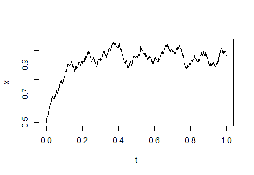
Plot some trajectories of an Ornstein-Uhlenbeck process with selected parameters and note the changes depending on parameter values.
Add the following parameter sets to their trajectories: = 20,
= 20,  = 1,
= 1,  = 1
= 1
- = 3, = 1, = 1
- = 20, = 3, = 5
- = 20, = 3, = 1
- Ornstein-Uhlenbeck process is used for example in interest rates modelling. Vasicek model assumes that the instantaneous interest rate (practically - when analysing real data - interest rate with a short maturity) follows an Ornstein-Uhlenbeck process.
In paper Athanasios Episcopos: Further evidence on alternative continuous time models of the short-term interest rate. Journal of International Financial Markets, Institutions and Money 10 (2000) 199-212 the author estimates interest rate models. The general model which he considered isSpecial choices of some of the parameters lead to concrete models, one of them is also the Vasicek model. Results for New Zealand (estimated are based on monthly data, from April 1986 - April 1998) can be seen in the following table, taken from the paper: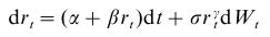 Source: (Episcopos, 2000)
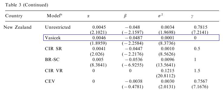
- The process is written in another parametization. Write it in terms of the parameters , , . What is the equilibrium level, to which the interest rate reverts?
- Simulate future behaviour of the interest rate using the estimated parameters of the Vasicek model. Into one graph, plot several sample paths starting from the same initial value.
- The process is written in another parametization. Write it in terms of the parameters
:: Expected value of a stochastic process ::
We are interested in the expected value of the Ornestein-Uhlenbeck process:- Using the same idea as in lecture for geometric Brownian motion, we derive the ordinary differential equation for the expected value at time t
- By solving this ODE we find the expected value
:: Exercises (2) ::
- Consider the expected value of the Ornstein Uhlenbeck process as a function of time. What is its limit as time approaches infinity? How does its behviour depend on the parameters of the process?
- Suppose that the interest rate follows the Vasicek model with the parameters given above in the table with estimates for New Zealand. Plot the expected value of the interest rate in the future for different initial values and observe the convergence.
- For what values of the parameters we would observe a higher speed of the convergence. Give a concrete example and modify the previous plot.
:: Ito lemma ::
As a revision from earlier courses, we compute the differential of a process
:: Exercises (3) ::
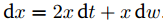
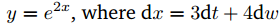
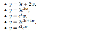
- Find the differential of a stochastic process
:: Exercises (3) ::
- Find the differentials of the stochastic processes
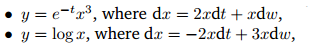
- Find the differentials of the stochastic processes
- Solving stochastic differential equations.In certain cases we are able to solve a given
stochastic differential equation. The following problems show some of the methods that can be used -
guessing a form of the solution (and determining the coefficients) and substitution leading to an equation
which is easier to solve.
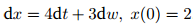
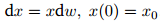
- Solve the following stochastic differential equation, i.e., find a process which satisfies the given
SDE and the initial condition:
Hint: The solution is a shifted Brownian motion.
- Solve the equation
using the following two methods:
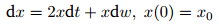
- Note that this is a special case of a geometric Brownian motion; hence write a general form of a GBM, compute its differential and match the coefficients.
- Alternatively, make a substitution y = log x, find the stochastic differential equation for y, solve it and finally express the original process x.
- (Exam, 2013) Solve the equation
- Use a substitution
to solve the equation

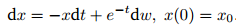
- Solve the following stochastic differential equation, i.e., find a process which satisfies the given
SDE and the initial condition:
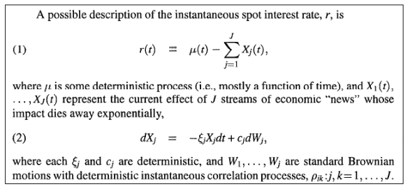
- Paper Babbs, S. H., & Nowman, K. B. (1999). Kalman filtering of generalized
Vasicek term structure models. Journal of Financial and Quantitative Analysis 34 (01),
115-130suggests the following model for the interest rate:
Explain the claim "whose impact dies away exponentially" by computing the expected value of the factor.
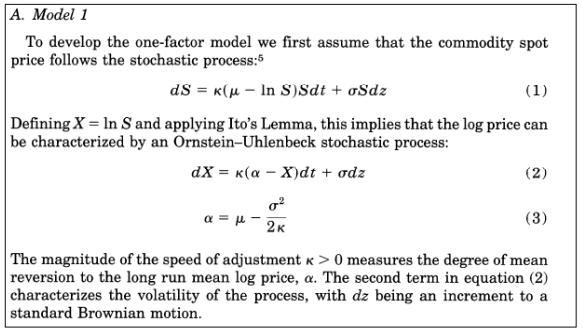
- In paper Schwartz, E. S. (1997). The stochastic behavior of commodity prices: Implications
for valuation and hedging. The Journal of Finance, 52(3), 923-973, the author
suggests several models for commodities prices, one of the is the following:
Derive that equation (1) implies that for the logaritm of the price we have the expressions (2), (3).
-
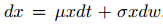
Suppose that x follows a geometric Brownian motion
- Define Show that the stochastic differential equation for y has again the form
 and determine
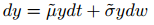

- Compute the probability that
- Define
Financial derivatives - exercises
Beáta Stehlíková, FMFI UK Bratislava
E-mail: stehlikova@pc2.iam.fmph.uniba.sk
Web: http://www.iam.fmph.uniba.sk/institute/stehlikova/
Beáta Stehlíková, FMFI UK Bratislava
E-mail: stehlikova@pc2.iam.fmph.uniba.sk
Web: http://www.iam.fmph.uniba.sk/institute/stehlikova/