Numerical solution of the Black-Scholes PDE
:: Why a numerical solution ::
- Why are we going to solve the equation numerically, when we have its explicit solution?
- Explicit solution is known to a European call and put options. For other derivatives, such a formula does not have to exist. However, a numerical solution is always possible.
- We firstly use numerical schemes for a case, for which we have an exact solution available. The advantage is that we can check the precision of the results which we obtain.
:: Transformation of the Black-Scholes equation ::
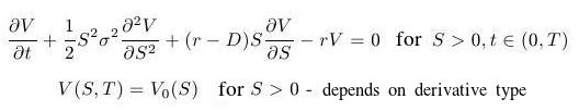
- Black-Scholes equation
- is it a parabolic PDE, which can be transformed to a heat equation with a given initial condition.
- Transformation of variables
- We have a terminal condition at time T (expiration time), not an initial one. This is solved by transformation
This means that the new variable (instead of original t denoting time) can be interpreted as time remaining to expiration.

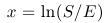
- Variable S (stock price) is positive. Variable, taking all real values, is obtained by taking logarithms. The new variable is therefore
Values of x close to zero correspond to stock prices that are close to the exercise price of the option. Negative value of x correspond to stock prices lower than the exercise price; positive values of x correspond to stock prices higher that the exercise price. It would be sufficient to take a logarithm of the price, but - as we will see later - this will be more convenient from a numerical point of view.
- We have a terminal condition at time T (expiration time), not an initial one. This is solved by transformation
- Transformation to heat equation
- The equation, obtained using the trasformations above, is a
parabolic equation, already with constant coefficients. This equation
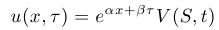
can be transformed to a heat equation by means of a transformation
where the constants are determined in such a way that the transformation leads to a heat equation. The correct choice of the constants is:
 Leads to
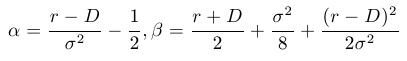
- The equation, obtained using the trasformations above, is a
parabolic equation, already with constant coefficients. This equation
can be transformed to a heat equation by means of a transformation
- Transformation of the terminal condition:

- By solving this heat equation and doing backwards transformations we obtain explicit Black-Scholes formulae, which we used earlier. However, now we want to solve this PDE numerically.
:: Discretization ::
- Variable x is from an unbounded interval, it attains values
from minus infinity to plus infinity. Numerically we are going to solve
the problem for x from a bounded interval [-L, L], where L is a sufficiently large number.
Note that this interval [-L, L] is not changed when considering an option with another exercise price. The suitable grid points S are obtained thanks to the transformation x = ln(S/E) which we have used instead of a simple logarithmic transformation x = ln(S).
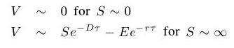
We need to impose boundary conditions for x = -L and x = L. These value of x correspond to stock prices which are very small, close to zero (the case of x = -L) and prices which are very high and approach infinity (the case of x = L). For these limiting values we will use the following approximations:
- Further, we have to discretize the heat equation. There are two basic possibilities:
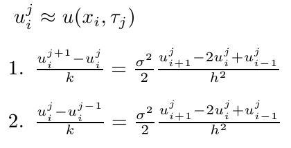
The first approach (explicit scheme) seems to be easier. We have an initial condition. Using these values, we compute the second time level. These are used to compute the next time level, etc. However, to ensure a convergence of the method, a certain condition on time and space steps is required. The condition may practically lead to a necessity of using a very small time step - because of a convergence, not because that we actually need the solution in so many close times.
The second approach (implicit scheme) leads to solving a system of linear equations on each time level.
:: Implicit scheme for a call option ::
-
We choose option parameters:
E <- 50
r <- 0.04
D <- 0.12
sigma <- 0.4
- We choose the parameter L which defines the space domain, on which we will compute a numerical solution:
L <- 2
and parameters of the partitions:n <- 20 h <- L/n T <- 1 m <- 12 k <- T/m
- Constants needed for the transformation of the equation:
alpha <- (r-D)/(sigma^2) - 0.5
beta <- (r+D)/2 + (sigma^2)/8 + ((r-D)^2)/(2*sigma^2)
- Boundary conditions for the transformed equation:
phi <- function(tau) 0
psi <- function(tau) E*exp(alpha*L + beta*tau)*(exp(L - D*tau) - exp(-r*tau))
and the initial condition:u0 <- function(x) E*exp(alpha*x)*pmax(0, exp(x)-1)
- We create a matrix, to which we will instert our numerical solution:
sol <- matrix(0, nrow=2*n + 1, ncol=m+1)
and grid points in time and in space:x <- seq(from=-L, by=h, to=L) tau <- seq(from=0, by=k, to=T)
Your task: Insert the boundary conditions and the initial condition into the matrix.
- To compute each of the time levels, we need to solve a system
of linear equations. Now we define the variables which appear in the
tridiagonal matrix of this system:
a <-  -0.5*(sigma^2)*k/(h^2)
b <-  1 - 2*a
When computing the first time level (the values at time k), we have the following right hand side:rhs <- sol[c(2:(2*n)),1] rhs[1] <- rhs[1] - a*phi(k) rhs[2*n-1] <- rhs[2*n-1] - a*psi(k)
Firstly, we will use the Gauss-Seidel method to solve this system of equations.You can use the function defined as follows, which solves a special symmetric tridiagonal system with a above and below the diagonal and b on the diagonal (rhs is the right hand side of the system, v0 is the initial iteration and N is number of iterations.
gs <- function(a,b,rhs,v0,eps,N) {
  n.system <- length(v0)
  v <- v0
  for (iter in 1:N) {
    v[1] <- (rhs[1] - a*v[2])/b
    for (i in 2:(n.system-1)) v[i] <- (rhs[i] - a*(v[i-1] + v[i+1]))/b
    v[n.system] <- (rhs[n.system] - a*v[n.system - 1])/b
  }
  gs <- v
}
Your tasks:- Compute the solution on the first time level and insert it into the solution matrix (as the initial approximation you can tke the values from the previous time level; choose a criterion for stopping iterations)
- Transform the solution into the solution of the Black-Scholes equation.
- Write a loop to compute the solution for each time level.
- Compare with the exact values from the Black-Scholes formula.
A sample output: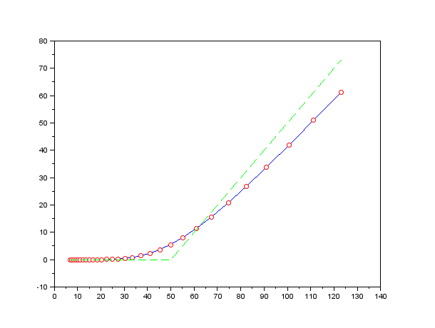
:: SOR method ::
- Adjust the function gs to create a new function sor, which has one additional parameter omega
and uses successiv over relaxation (SOR) method to numerically compute
solution to the same system of equations. Then, use it to find
numerical values of option prices.
Note: The only change in the main code will be calling the function sor instead of the function gs.
-
For the first element of the solution:
vOld <-  v[1]
vGS <- (rhs[1] - a*v[2])/b;
v[1] <- omega*vGS + (1-omega)*vOld
In the same way for other ones.
:: Comparison of numerical pricing: European vs. American option ::
European option - algorithm for the transformed function u- We compute the boundary conditions and insert them into the solution matrix.
- We compute the initial condition and insert it into the solution matrix.
- Computation of the next time level - SOR method:
- Initial approximation: we can take the values from the previous time level
- Condition for stopping the iterations - norm of the residue, difference between two iterations, number of iterations
- Computation of a new iteration using the SOR method - we repeat until the condition for stopping the iteration is not satisfied, the we move to the next time level
- We compute the boundary conditions. The solution has to lie above the transformed payoff => we compute max(boundary condition, transformed payoff) and insert it into the solution matrix.
- We compute the initial condition and insert it into the solution matrix.
- Computation of the next time level - PSOR method (projected SOR method)
- Initial approximation - we want one that is close to solution, so that we do not have to compute many iterations: we compare the values from the previous time level with the transformed payoff => we take max(previous time level, transformed payoff)
- Condition for stopping the iterations - norm of a residue cannot be used, since we do not compute a solution to a system of equations, we use the difference of two subsequent iterations or a given number of iterations
- Computation of a new iteration using the PSOR method - we compute the i-th elemts of the vector using SOR method and compare it with the transformed payoff => we take max(SOR iteration, transformed payoff) and compute the next element - we repeat until the condition for stopping the iteration is not satisfied, the we move to the next time level
:: Practice problems ::
- Optimal omega for the SOR method. Prove that the eigenvalues of the matrix
are
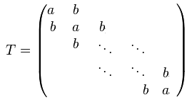 for k=1,2,...,n. Use this result to derive the optimal omega for SOR method applied to numerical solution of the Black-Scholes equation. The optimal omega shoud be expressed as a function of gamma defined in the lectures (depending on time and space step, and on stock volatility). Hint: Prove it firstly for a=0, b=1 and them show the relation between the eigenvalues of this matrix and the original one.
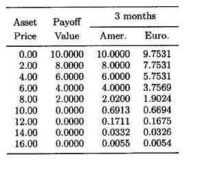
- Implement the numerical pricing of an American put. Use it to solve the following pricing problem:
The stock price follows a geometrical Brownian motion with parameters
 =0.20,
  =0.40. The stock does not pay dividends. Interest rate equals 10 percent. Compute the price of a put option with expiration in 3 months and exercise pirce 10 USD for the following stock pricces: 0, 2, 4, 6, 8, 10, 12, 14, 16 USD. Round the results to 4 decimal places.
You can check your results with those below:
=0.40. The stock does not pay dividends. Interest rate equals 10 percent. Compute the price of a put option with expiration in 3 months and exercise pirce 10 USD for the following stock pricces: 0, 2, 4, 6, 8, 10, 12, 14, 16 USD. Round the results to 4 decimal places.
You can check your results with those below:
Beáta Stehlíková, FMFI UK Bratislava
E-mail: stehlikova@pc2.iam.fmph.uniba.sk
Web: http://www.iam.fmph.uniba.sk/institute/stehlikova/