Random processes I.
Wiener process, Brownian motion, GBM
:: Stochastic character of financial variables ::
-
From the trajectories of stock prices (also other financial variables - interest rate, exchange rates, etc.) we see that it cannot be described by a deterministic function. Therefore, stochastic processes are used in the modelling. .
-
Left: trend (stock price, 5 years time frame), right: fluctuations (stock price, time frame of a couple of hours)
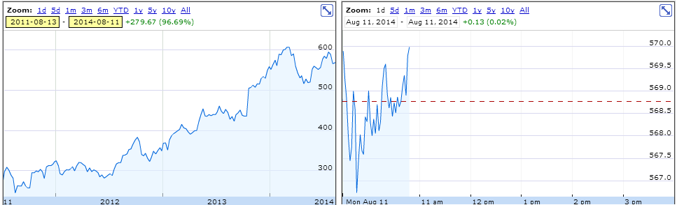 Source: http://finance.google.com
:: Wiener process and Brownian motion ::

| Download [ex02processes.sce] - Scilab file with the code shown below; we will write more |
-
The basic process, used to derive more complicated ones, is a Wienerov proces. Recall its definition:
Random process {W(t), tIn what follow, we done a Wiener process by w. 0} is called a Wiener process, if
- the increments
W(t+
 ) - W(t) have a normal distribution with zero expected value and variance equal to ,
- for every partition 0 = t0
 t1 ... tn, the increments
Wti+1 - Wti nare independent random variables, with distribution given in the previous points ,
t1 ... tn, the increments
Wti+1 - Wti nare independent random variables, with distribution given in the previous points ,
- W(0)=0,
- trajectories are continuous.
- the increments
W(t+
-
How to obtain a sample path (trajectory) of a Wiener process
- We will generate an approximation - values at discrete points of the form (time, value of the process) which we join by line segments.
- The times will be 0,,2, . . ., where is a sufficiently small time step.
- Value at time 0 is equal to 0.
- Increment on the interval [k, (k + 1)] is a random variable with zero expected value and variance equal to .
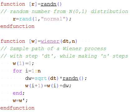
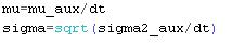
In Scilab we firstly define auxiliary functions:
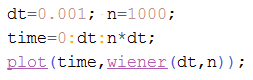
Now we can plot a trajectory:
Plot several trajectories of a Wiener process into one plot. A sample output:
-
By adding a linear trend to a multiple of a Wiener process:
we obtain a process which is known as a Brownian motion.
If the parameter
 is zero, the resulting graph is a line. For a nonzero value of , there are random fluctuations added to this linear trend.
In Scilab - for example:
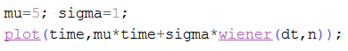
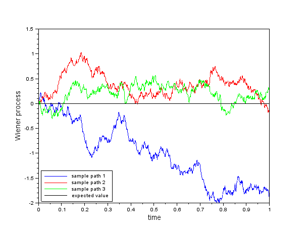
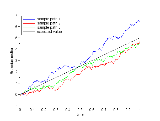
Plot several trajectories of a Wiener process into one plot and add the expected value. A sample output:
:: Exercises (1) ::
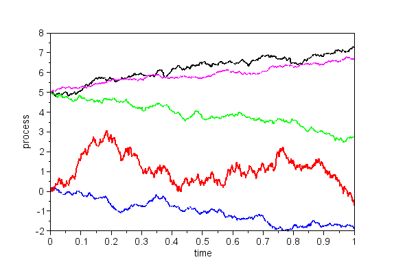
- Modify parameters of a Brownian motion and note the influence on typical trajectories. Then, add the processes
- x1(t)=w(t)
- x2(t)=3*w(t)
- x3(t)=5+2*t+w(t)
- x4(t)=5+2*t+0.5*w(t)
- x5(t)=5-3*t+w(t)
:: Geometric Brownian motion ::
-
Geometric Brownian motion is defined as:
where x0 is the value of the process at time 0.
- Simulating in Scilab:

-
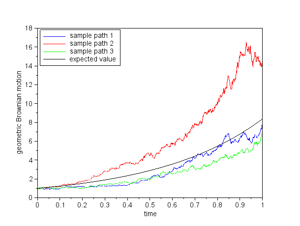
Sample paths of a geometric Brownian motion:
Make a similar plot.
:: Modelling stock prices by mean of a geometric Brownian motion ::
-
GBM as a model for the stock price S:
-
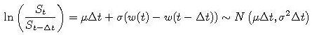
Recall from the lecture: If the stock price S follows a GBM, then for the returns we have
hence the returns are independent random variables with the distribution given above.
:: Exercises (2) ::
Recall from the probability course the definition and basic properties of a lognormal distribution:- Random variable X has a lognormal distribution, if its logarithm ln(X) has a normal distribution
 .
.
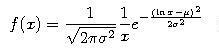
- Probability density function of a lognormal random variable X is given by
(for positive x, otherwise it is zero)
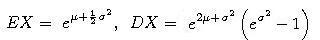
- Expected value and variance of a random variable X with lognormal distribution are given by

| Download [ex02stock.sce] - Scilab file with an outline of solution to the following problems and some useful functions |
Suppose that the stock price follows a GBM with parameters
 = 0.30,
 = 0.25
and that its current price is 150 USD.
= 0.25
and that its current price is 150 USD.
- Plot the probability density function of the stock price in one month. To check your computation, compare it with a histogram of simulated values of the stock price in one month.
- Compute the probability that the price in one month will be lower than 140 USD?
- What it expected value of the 1/4-year return? What is the probability of this return to be negative?
:: Estimating the parameters of the GBM from stock prices ::

| Download [amzn.txt] and [ex02data.sce] - stock price data in text file and Scilab file with the code given below and the outline of estimation |
How to obtain estimates of parameters - we use the procedure from the lecture (cf. the slides) and replicate the results
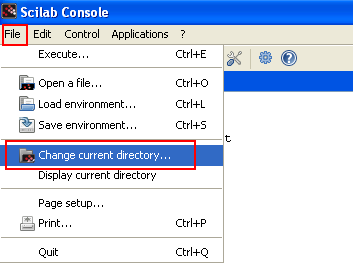
- Firstly, set the working directory, so that it contains the data.
- Read the data to Scilab. These are daily data, so we set the value of the variable dt, measuring the length of a time step in years, to 1/252.
- We define the returns - we create a vector of returns v using the formula above
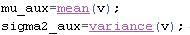
- We know that these returns have a normal distribution. Furthermore, we know that the expected value of a normal distribution is estimated by a sample mean and the variance is estimated by a sample variance.
Therefore we compute the mean and the sample variance of the value in vector v - these will be estimates of the quantities
 and
and 
- Finally, we compute the estimates of the parameters
 and
and  :
:
:: Practice problems ::
-
Denote by tM the time, in which the sample path of the Wiener process achieved its maximum on
the time interval [0, 1] Plot a histogram by simulating the realizations of the random variable tM.
A trajectory of a Wiener process and corresponding value of tM is shown below, together with a sample histogram.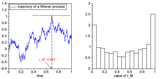
- Let w be a Wiener process; define B(t) = w(t) - t w(1) for time t in interval [0, 1]. It is known as Brownian bridge.
- Plot some sample paths of the process and explain its name.
- Compute its variance at time t and sketch its behaviour as a function of time. To check your computation - what does the result have to be for t=0 and t=1?
- More practice problems in the course notes
Financial derivatives, 2014
Beáta Stehlíková, FMFI UK Bratislava
E-mail: stehlikova@pc2.iam.fmph.uniba.sk
Web: http://www.iam.fmph.uniba.sk/institute/stehlikova/
Beáta Stehlíková, FMFI UK Bratislava
E-mail: stehlikova@pc2.iam.fmph.uniba.sk
Web: http://www.iam.fmph.uniba.sk/institute/stehlikova/