:: One-factor short rate model ::

• Interest rates - for example Euribor:
  
• Short rate - instantaneous interest rate, an interest rate with a short maturity is used as a proxy
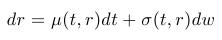
• The short rate is modelled by a stochastic differential equation:
  
  hence trend in the short rate evolution + random fluctuations around the trend
• One-factor model - one stochastic differential equation for r, i.e., one source of randomness in the short rate evolution (one Wiener process).

:: Vasicek model :::

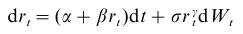
• Stochastic differential equation for the short rate:
  
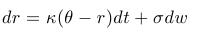
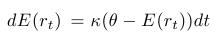
• Mean-reversion property - for the expected value we have
  
• Volatility is constant, it does not depend on the current level of the short rate
• We have already encountered the process, used to model the short rate in the Vasicek model in exercises dealing with stochastic differential equations. Recall the dependence of the process on its parameters using Exercise (1)/1.

:: Probability distribution of the short rate ::

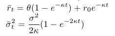
• See the lectures: we computed the conditional distribution of the short rate, when its value r₀ at time t = 0 - it is a normal distribution with parameters
  
• Knowledge of this distribution enables us to:
  • simulate a trajectory of a process for given parameters and an initial value of the interest rate
  • estimate parameters of the model from the data
• Note: There are different notations for the linear function in the drift, which can be seen in the literature; therefore it is necessary to always check what is the parametrization of the drift.

:: Exercises (1) ::

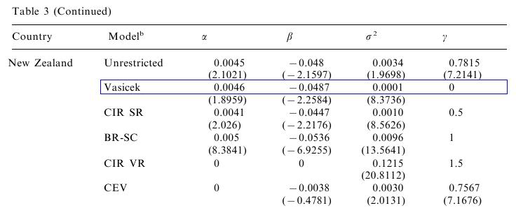
1. As in the exercises dealing with stochastic differential equations, we are going to use parameters from the paper Athanasios Episcopos: Further evidence on alternative continuous time models of the short-term interest rate. Journal of International Financial Markets, Institutions and Money 10 (2000) 199-212, where the author estimated interest rate modes. The general model, which he considered, was
   
   Again, we consider the results for New Zealand:
   
   
   
   • Recall the transformation of these parameters to obtain the process expressed in terms of , , .
     
     
   • Before, we generated trajectories using the Euler-Maruyama approximation. Compare the probability distribution of the interest rate obtained from this approximation with the exact distribution, if the time step is 1 day, 1 week, 1 month, 1 year. In what follows, we will use the exact distribution.
     
     
   • Suppose the the interest rate today is 4.5 percent. What is its expected value in 1 week, 1 month, 1 year? Construct also confidence intervals for these values (expected value +/- 2 * standard deviation).
     
     
   • What is the limiting distribution of the interest rate? Plot a graph of the density of this limiting distribution. Add graphs of densities of probability distributions of the interest rate in 1 month, 1 year, ... - so that the convergence of these densities to the limiting density can be observed.

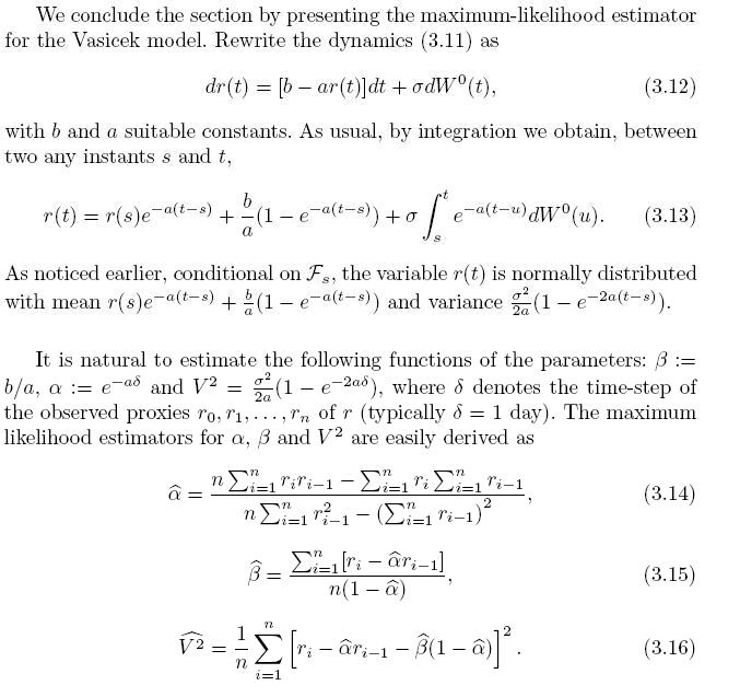
:: Maximum likelihood methods for estimatig the parameters ::

• Conditional distribution of interest rates is normal, therefore the likelihood function is a product of densities of normal distributions. The maximum likelihood estimated can be explicitly expressed.
  
  
• Damiano Brigo, Fabio Mercurio: Interest Rate Models - Theory and Practice. Second Edition. Springer, 2007. Chapter 3.1.2, pp. 61-62:
  
  Source: [books.google.com]
  
  
• You may find this following script convenient; there are formulae from the text above: [vasicekMLE.sce]

:: Exercises (2) ::

1. How to obtain the estimates of , , from the results given above? Derive the transformation.
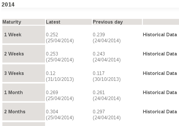
2. Use the data from the file euro2014q1.txt which contains the values of 1-month Euribor (which we will use as a proxy for the short rate), the data are from the first quarter of the year 2014 (note that you need to to divide them by 100).
   • Estimate the parameters of the model.
   • What is the estimated equilibrium level (i.e., to what value the process reverts) of the short rate? Plot the graph of the data together with the estimated equilibrium rate.
   • Add the expected value of the interest rate into the previous plot.
   • What is the probability that the interest rate at the end of the year will be below the equilibrium level?

:: Practice problems ::

• Download the interest rate data (for example, 3M treasury bills, Euribor with short maturity, etc.) from a selected time interval. Plot their evolution in time. Possible sources of data:
  • Federal Reserve Statistical Release
  • Euribor.org
  • Bank of Canada
• Estimate parameters of the Vasicek model and transform them to the parameters, , .
• For a given initial value of the interest rate (for example, the last value from the data), plot into one graph its future expected value, confidence intervals for each time and a couple of trajectories.
• Find the limiting distribution of the short rate.

---